When a Firm Is on the Inelastic Segment of Its Demand Curve, It Can:

10.2 The Monopoly Model

Learning Objectives

1. Explicate the relationship between price and marginal revenue when a firm faces a down-sloping need curve.
2. Explain the relationship between marginal revenue and elasticity along a linear demand curve.
3. Apply the marginal determination rule to explain how a monopoly maximizes turn a profit.

Analyzing choices is a more complex challenge for a monopoly firm than for a perfectly competitive firm. Later all, a competitive firm takes the market price every bit given and determines its profit-maximizing output. Considering a monopoly has its market all to itself, it tin can determine not merely its output only its price as well. What kinds of price and output choices will such a firm brand?

We will answer that question in the context of the marginal decision rule: a firm will produce boosted units of a good until marginal acquirement equals marginal toll. To use that dominion to a monopoly firm, we must first investigate the special relationship between demand and marginal acquirement for a monopoly.

Monopoly and Market Demand

Because a monopoly firm has its market all to itself, it faces the market place demand bend. Figure 10.two "Perfect Competition Versus Monopoly" compares the demand situations faced by a monopoly and a perfectly competitive firm. In Panel (a), the equilibrium price for a perfectly competitive firm is determined by the intersection of the demand and supply curves. The marketplace supply bend is found simply by summing the supply curves of individual firms. Those, in plow, consist of the portions of marginal cost curves that prevarication above the average variable price curves. The marginal cost curve, MC, for a single firm is illustrated. Observe the interruption in the horizontal axis indicating that the quantity produced past a single business firm is a trivially small fraction of the whole. In the perfectly competitive model, ane firm has nothing to do with the determination of the market price. Each firm in a perfectly competitive industry faces a horizontal demand curve defined by the market price.

Figure 10.two Perfect Competition Versus Monopoly

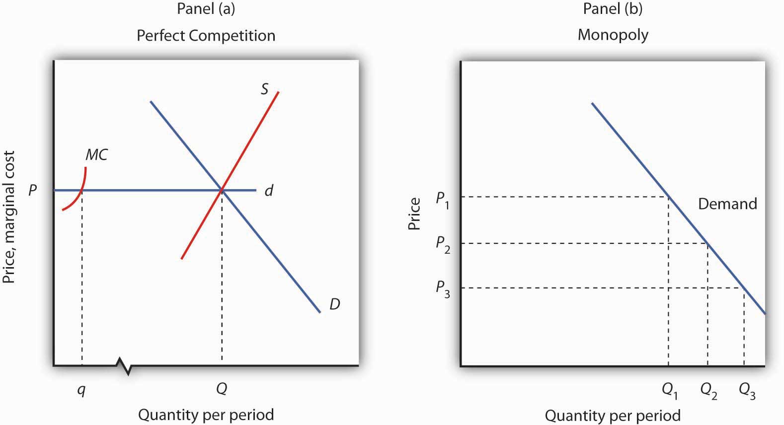
Console (a) shows the determination of equilibrium price and output in a perfectly competitive market place. A typical firm with marginal toll bend MC is a toll taker, choosing to produce quantity q at the equilibrium toll P. In Panel (b) a monopoly faces a downward-sloping marketplace demand curve. As a turn a profit maximizer, it determines its profit-maximizing output. Once it determines that quantity, however, the price at which it tin sell that output is found from the demand curve. The monopoly business firm can sell additional units simply past lowering price. The perfectly competitive house, past dissimilarity, tin sell whatever quantity it wants at the market price.

Contrast the situation shown in Panel (a) with the one faced by the monopoly firm in Panel (b). Because it is the only supplier in the manufacture, the monopolist faces the down-sloping market place demand curve alone. Information technology may choose to produce any quantity. But, unlike the perfectly competitive firm, which can sell all it wants at the going market place toll, a monopolist can sell a greater quantity simply by cutting its price.

Suppose, for case, that a monopoly firm can sell quantity Q ₁ units at a price P ₁ in Panel (b). If it wants to increase its output to Q ₂ units—and sell that quantity—information technology must reduce its toll to P _ii. To sell quantity Q ₃ it would have to reduce the price to P _three. The monopoly firm may choose its price and output, only it is restricted to a combination of price and output that lies on the demand bend. It could not, for example, charge cost P ₁ and sell quantity Q _three. To be a price setter, a firm must face up a downward-sloping demand curve.

Total Revenue and Cost Elasticity

A house'south elasticity of demand with respect to price has of import implications for assessing the impact of a price change on full revenue. Likewise, the price elasticity of demand tin can be different at different points on a business firm'due south demand curve. In this section, we shall see why a monopoly house volition always select a toll in the elastic region of its need curve.

Suppose the demand curve facing a monopoly firm is given by Equation 10.ane, where Q is the quantity demanded per unit of fourth dimension and P is the price per unit:

This demand equation implies the demand schedule shown in Figure 10.3 "Demand, Elasticity, and Total Revenue". Total revenue for each quantity equals the quantity times the price at which that quantity is demanded. The monopoly firm'south total revenue curve is given in Console (b). Because a monopolist must cut the price of every unit of measurement in gild to increase sales, full revenue does non always increase as output rises. In this instance, total revenue reaches a maximum of $25 when 5 units are sold. Beyond 5 units, full revenue begins to decline.

Figure ten.iii Demand, Elasticity, and Total Acquirement

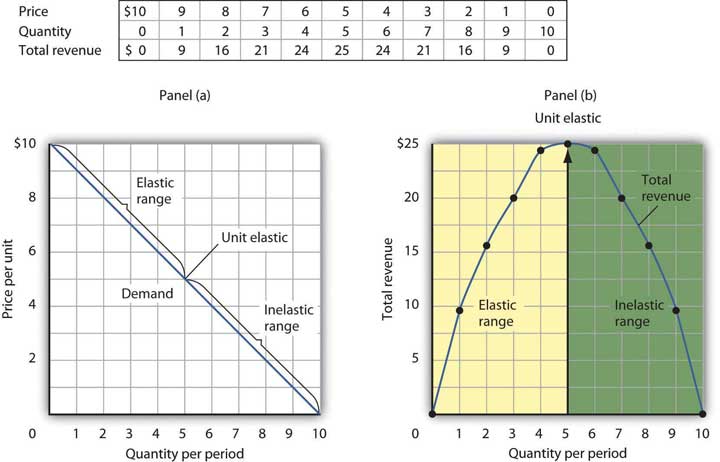
Suppose a monopolist faces the downwardly-sloping demand curve shown in Panel (a). In order to increase the quantity sold, it must cut the cost. Full acquirement is constitute by multiplying the price and quantity sold at each toll. Total revenue, plotted in Console (b), is maximized at $25, when the quantity sold is 5 units and the price is $five. At that signal on the demand curve, the toll elasticity of demand equals −1.

The demand curve in Console (a) of Figure 10.3 "Demand, Elasticity, and Total Acquirement" shows ranges of values of the price elasticity of demand. We have learned that cost elasticity varies forth a linear need curve in a special way: Need is price elastic at points in the upper one-half of the demand curve and price inelastic in the lower half of the demand curve. If demand is cost elastic, a price reduction increases total revenue. To sell an additional unit, a monopoly house must lower its price. The sale of one more unit will increase acquirement because the percentage increase in the quantity demanded exceeds the percentage decrease in the price. The rubberband range of the demand bend corresponds to the range over which the total revenue curve is rising in Panel (b) of Effigy 10.3 "Demand, Elasticity, and Total Revenue".

If demand is toll inelastic, a price reduction reduces total revenue because the percentage increase in the quantity demanded is less than the percentage decrease in the toll. Total acquirement falls as the firm sells additional units over the inelastic range of the demand curve. The downward-sloping portion of the full acquirement curve in Console (b) corresponds to the inelastic range of the need bend.

Finally, recall that the midpoint of a linear demand curve is the point at which demand becomes unit of measurement price rubberband. That point on the total revenue curve in Panel (b) corresponds to the betoken at which total revenue reaches a maximum.

The human relationship amid price elasticity, demand, and total revenue has an important implication for the selection of the profit-maximizing price and output: A monopoly business firm volition never choose a price and output in the inelastic range of the demand curve. Suppose, for instance, that the monopoly firm represented in Effigy ten.iii "Demand, Elasticity, and Full Revenue" is charging $3 and selling vii units. Its total revenue is thus $21. Considering this combination is in the inelastic portion of the demand bend, the firm could increase its full revenue past raising its toll. It could, at the same time, reduce its full toll. Raising price means reducing output; a reduction in output would reduce total cost. If the business firm is operating in the inelastic range of its demand curve, and then it is non maximizing profits. The firm could earn a higher turn a profit by raising price and reducing output. It will continue to raise its price until information technology is in the elastic portion of its demand curve. A profit-maximizing monopoly house will therefore select a price and output combination in the elastic range of its demand curve.

Of grade, the firm could choose a point at which demand is unit of measurement toll rubberband. At that point, total acquirement is maximized. But the business firm seeks to maximize profit, not total acquirement. A solution that maximizes total acquirement volition not maximize profit unless marginal cost is naught.

Demand and Marginal Acquirement

In the perfectly competitive case, the additional revenue a firm gains from selling an additional unit—its marginal revenue—is equal to the market cost. The firm's demand curve, which is a horizontal line at the market price, is also its marginal revenue curve. But a monopoly firm can sell an additional unit only by lowering the price. That fact complicates the relationship between the monopoly's demand curve and its marginal revenue.

Suppose the firm in Effigy ten.3 "Demand, Elasticity, and Total Acquirement" sells 2 units at a toll of $8 per unit. Its total acquirement is $sixteen. Now information technology wants to sell a third unit and wants to know the marginal revenue of that unit. To sell 3 units rather than ii, the firm must lower its price to $vii per unit. Total acquirement rises to $21. The marginal revenue of the tertiary unit of measurement is thus $v. But the price at which the business firm sells 3 units is $7. Marginal revenue is less than price.

To see why the marginal revenue of the third unit is less than its price, we need to examine more than advisedly how the sale of that unit of measurement affects the firm's revenues. The firm brings in $7 from the sale of the third unit. But selling the tertiary unit required the firm to accuse a price of $7 instead of the $8 the firm was charging for 2 units. Now the firm receives less for the first 2 units. The marginal acquirement of the third unit is the $7 the business firm receives for that unit minus the $one reduction in revenue for each of the starting time two units. The marginal acquirement of the third unit is thus $five. (In this affiliate we presume that the monopoly firm sells all units of output at the aforementioned price. In the next chapter, we will look at cases in which firms charge different prices to different customers.)

Marginal acquirement is less than cost for the monopoly house. Effigy 10.4 "Demand and Marginal Revenue" shows the relationship between demand and marginal revenue, based on the need curve introduced in Effigy x.3 "Need, Elasticity, and Total Revenue". As e'er, we follow the convention of plotting marginal values at the midpoints of the intervals.

Figure 10.4 Demand and Marginal Revenue

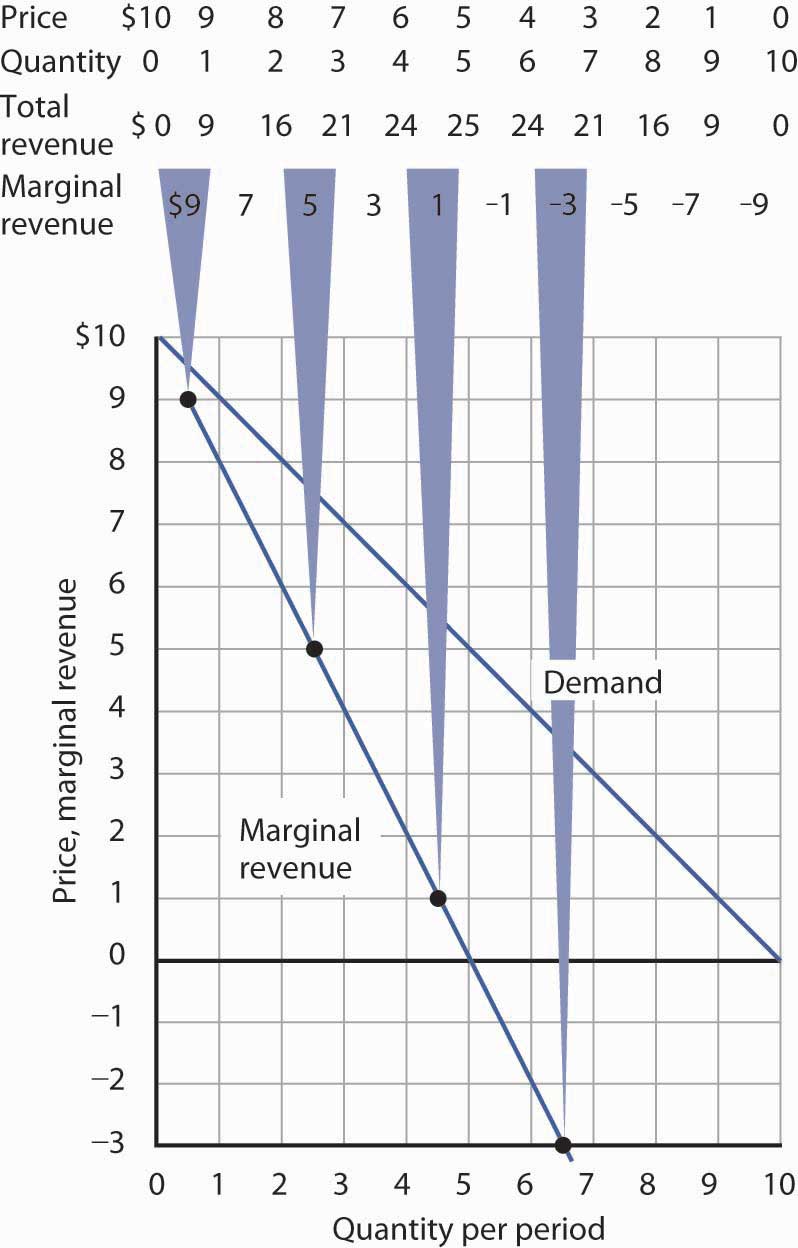
The marginal revenue bend for the monopoly firm lies below its need bend. It shows the additional acquirement gained from selling an additional unit of measurement. Notice that, equally always, marginal values are plotted at the midpoints of the respective intervals.

When the need curve is linear, equally in Figure 10.4 "Demand and Marginal Revenue", the marginal acquirement curve tin be placed co-ordinate to the post-obit rules: the marginal acquirement curve is always below the demand curve and the marginal revenue curve will bisect any horizontal line drawn betwixt the vertical axis and the demand curve. To put it another way, the marginal revenue curve will be twice as steep as the demand curve. The demand curve in Figure 10.4 "Demand and Marginal Revenue" is given by the equation $Q=10-P$ , which tin be written $P=10-Q$ . The marginal revenue curve is given by $P=\mathrm{ten}-2Q$ , which is twice as steep equally the demand curve.

The marginal acquirement and demand curves in Figure x.iv "Demand and Marginal Revenue" follow these rules. The marginal revenue curve lies beneath the demand curve, and information technology bisects any horizontal line drawn from the vertical centrality to the demand curve. At a price of $6, for example, the quantity demanded is iv. The marginal acquirement bend passes through two units at this price. At a price of 0, the quantity demanded is 10; the marginal revenue curve passes through v units at this point.

Just as there is a relationship between the firm'southward demand curve and the price elasticity of need, there is a relationship between its marginal revenue curve and elasticity. Where marginal revenue is positive, demand is price rubberband. Where marginal revenue is negative, need is price inelastic. Where marginal revenue is null, demand is unit of measurement price elastic.

When marginal acquirement is …	then need is …
positive,	price elastic.
negative,	cost inelastic.
zero,	unit of measurement price elastic.

A house would not produce an additional unit of output with negative marginal acquirement. And, assuming that the product of an additional unit has some price, a house would not produce the extra unit if it has nil marginal acquirement. Because a monopoly business firm volition mostly operate where marginal acquirement is positive, nosotros run into one time over again that information technology volition operate in the rubberband range of its need bend.

Monopoly Equilibrium: Applying the Marginal Decision Rule

Profit-maximizing behavior is e'er based on the marginal decision rule: Additional units of a adept should exist produced as long as the marginal revenue of an additional unit exceeds the marginal cost. The maximizing solution occurs where marginal revenue equals marginal cost. As always, firms seek to maximize economical profit, and costs are measured in the economic sense of opportunity cost.

Effigy 10.five "The Monopoly Solution" shows a demand curve and an associated marginal acquirement curve facing a monopoly firm. The marginal price bend is like those we derived earlier; it falls over the range of output in which the firm experiences increasing marginal returns, then rises equally the firm experiences diminishing marginal returns.

Figure 10.5 The Monopoly Solution

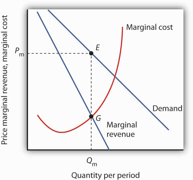
The monopoly firm maximizes profit by producing an output Q ₁₀₀₀ at bespeak Yard, where the marginal revenue and marginal cost curves intersect. Information technology sells this output at price P _m.

To decide the profit-maximizing output, nosotros note the quantity at which the firm's marginal acquirement and marginal toll curves intersect (Q _thousand in Figure 10.5 "The Monopoly Solution"). We read up from Q _m to the demand curve to find the price P _m at which the firm can sell Q _m units per menstruation. The profit-maximizing price and output are given by point E on the demand curve.

Thus we tin determine a monopoly firm's turn a profit-maximizing price and output by following three steps:

1. Make up one's mind the demand, marginal revenue, and marginal cost curves.
2. Select the output level at which the marginal acquirement and marginal toll curves intersect.
3. Make up one's mind from the need bend the cost at which that output can be sold.

Figure 10.6 Computing Monopoly Turn a profit

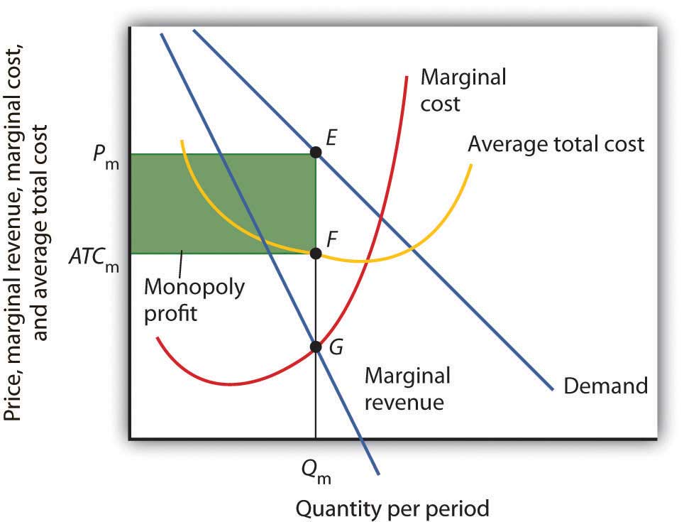
A monopoly firm'south profit per unit is the difference between price and average full cost. Total profit equals profit per unit of measurement times the quantity produced. Total profit is given past the area of the shaded rectangle ATC _thousand P _mEF.

Once we have determined the monopoly firm'south price and output, we can determine its economic profit by calculation the house's average total cost curve to the graph showing demand, marginal revenue, and marginal cost, as shown in Figure ten.six "Computing Monopoly Profit". The boilerplate total cost (ATC) at an output of Q _chiliad units is ATC _m. The firm's profit per unit is thus P _m - ATC _m. Total profit is institute by multiplying the firm's output, Q _m, past turn a profit per unit, so total profit equals Q _thousand(P _grand - ATC _m)—the area of the shaded rectangle in Figure 10.vi "Computing Monopoly Profit".

Heads Up!

Dispelling Myths Virtually Monopoly

3 mutual misconceptions nigh monopoly are:

1. Considering there are no rivals selling the products of monopoly firms, they can charge whatsoever they desire.
2. Monopolists volition charge whatever the market volition deport.
3. Considering monopoly firms accept the market to themselves, they are guaranteed huge profits.

Every bit Figure x.5 "The Monopoly Solution" shows, once the monopoly firm decides on the number of units of output that will maximize profit, the toll at which it tin sell that many units is institute by "reading off" the demand curve the price associated with that many units. If it tries to sell Q _m units of output for more than than P _m, some of its output will become unsold. The monopoly business firm tin can set its cost, just is restricted to price and output combinations that lie on its demand curve. It cannot just "charge whatever it wants." And if it charges "all the market will bear," information technology will sell either 0 or, at about, 1 unit of output.

Neither is the monopoly firm guaranteed a profit. Consider Figure 10.vi "Calculating Monopoly Profit". Suppose the average full price curve, instead of lying below the demand bend for some output levels every bit shown, were instead everywhere in a higher place the demand bend. In that case, the monopoly volition incur losses no affair what price it chooses, since average full price volition always exist greater than any price it might charge. Every bit is the case for perfect contest, the monopoly firm can keep producing in the curt run so long as price exceeds average variable cost. In the long run, information technology volition stay in business organization only if it can cover all of its costs.

Central Takeaways

• If a firm faces a downwardly-sloping demand bend, marginal revenue is less than price.
• Marginal revenue is positive in the elastic range of a demand bend, negative in the inelastic range, and zero where demand is unit price rubberband.
• If a monopoly house faces a linear demand curve, its marginal acquirement curve is also linear, lies beneath the demand curve, and bisects whatever horizontal line drawn from the vertical axis to the need curve.
• To maximize turn a profit or minimize losses, a monopoly firm produces the quantity at which marginal cost equals marginal revenue. Its toll is given by the indicate on the demand curve that corresponds to this quantity.

Try It!

The Troll Road Company is because building a toll route. It estimates that its linear need bend is every bit shown beneath. Assume that the fixed cost of the road is $0.5 meg per year. Maintenance costs, which are the only other costs of the road, are also given in the table.

Tolls per trip	$1.00	0.90	0.80	0.70	0.60	0.fifty
Number of trips per year (in millions)	i	2	3	four	v	half dozen
Maintenance toll per year (in millions)	$0.7	1.2	1.8	ii.ix	four.ii	6.0

1. Using the midpoint convention, compute the profit-maximizing level of output.
2. Using the midpoint convention, what price volition the company charge?
3. What is marginal revenue at the profit-maximizing output level? How does marginal revenue compare to price?

Case in Bespeak: Profit-Maximizing Sports Teams

Love of the game? Dear of the metropolis? Are those the factors that influence owners of professional sports teams in setting admissions prices? Four economists at the University of Vancouver have what they recollect is the respond for one grouping of teams: professional hockey teams prepare access prices at levels that maximize their profits. They regard hockey teams as monopoly firms and use the monopoly model to examine the squad'due south behavior.

The economists, Donald G. Ferguson, Kenneth M. Stewart, John Colin H. Jones, and Andre Le Dressay, used information from three seasons to judge demand and marginal acquirement curves facing each team in the National Hockey League. They found that demand for a team'south tickets is affected by population and income in the team's home city, the team's standing in the National Hockey League, and the number of superstars on the team.

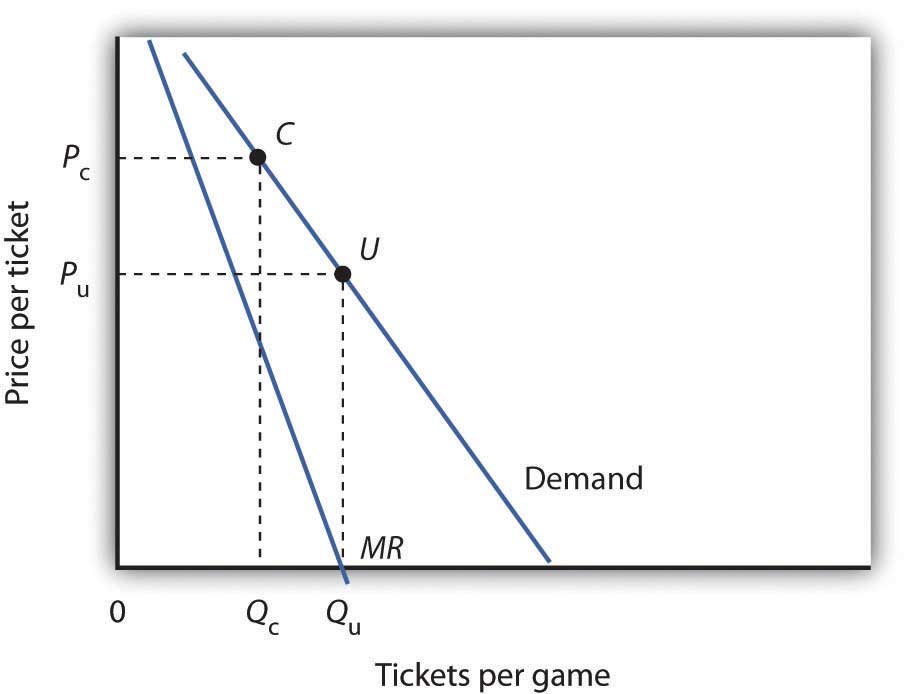
Because a sports team's costs practice non vary significantly with the number of fans who attend a given game, the economists assumed that marginal cost is zero. The profit-maximizing number of seats sold per game is thus the quantity at which marginal revenue is cypher, provided a team'due south stadium is large enough to hold that quantity of fans. This unconstrained quantity is labeled Q _u, with a corresponding price P _u in the graph.

Stadium size and the demand bend facing a team might prevent the squad from selling the profit-maximizing quantity of tickets. If its stadium holds only Q _c fans, for example, the team volition sell that many tickets at price P _c; its marginal revenue is positive at that quantity. Economical theory thus predicts that the marginal revenue for teams that consistently sell out their games will exist positive, and the marginal revenue for other teams will be zero.

The economists' statistical results were consistent with the theory. They found that teams that do non typically sell out their games operate at a quantity at which marginal revenue is about zero and that teams with sellouts have positive marginal revenue. "It's clear that these teams are very sophisticated in their use of pricing to maximize profits," Mr. Ferguson said.

Non all studies of sporting event pricing have confirmed this conclusion. While a study of major league baseball ticket pricing by Leo Kahane and Stephen Shmanske and one of baseball leap training game tickets by Michael Donihue, David Findlay, and Peter Newberry suggested that tickets are priced where demand is unit of measurement elastic, another studies of ticket pricing of sporting events have found that tickets are priced in the inelastic region of the need curve. On its face, this would hateful that squad owners were not maximizing profits. Why would team owners do this? Are they actually charging too footling? To fans, information technology certainly may not seem and then!

While some have argued that owners want to please fans by selling tickets for less than the profit-maximizing price, others argue they practise then for possible political considerations, for example, keeping prices below the profit-maximizing level could aid when they are request for subsidies for building new stadiums. In line with the notion that team owners practice deport like other turn a profit-maximizing firms, another line of research, for instance, that proposed by Anthony Krautmann and David Berri, has been to recognize that owners also get revenue from selling concessions so that getting more than fans at the game may boost revenue from other sources.

Sources: Michael R. Donihue, David W. Findlay, and Peter Due west. Newberry, "An Analysis of Attendance at Major League Baseball Spring Games," Periodical of Sports Economics eight:ane (Feb 2007): 39–61; Donald G. Ferguson et al., "The Pricing of Sports Events: Practice Teams Maximize Profit?" Journal of Industrial Economics 39:3 (March 1991): 297–310 and personal interview; Leo Kahane and Stephen Shmanske, "Team Roster Turnover and Attendance in Major League Baseball," Practical Economics 29 (1997): 425–431; and Anthony C. Krautmann and David J. Berri, "Can We Notice Information technology at the Concessions?" Journal of Sports Economics 8:ii (Apr 2007): 183–191.

Answer to Try It! Trouble

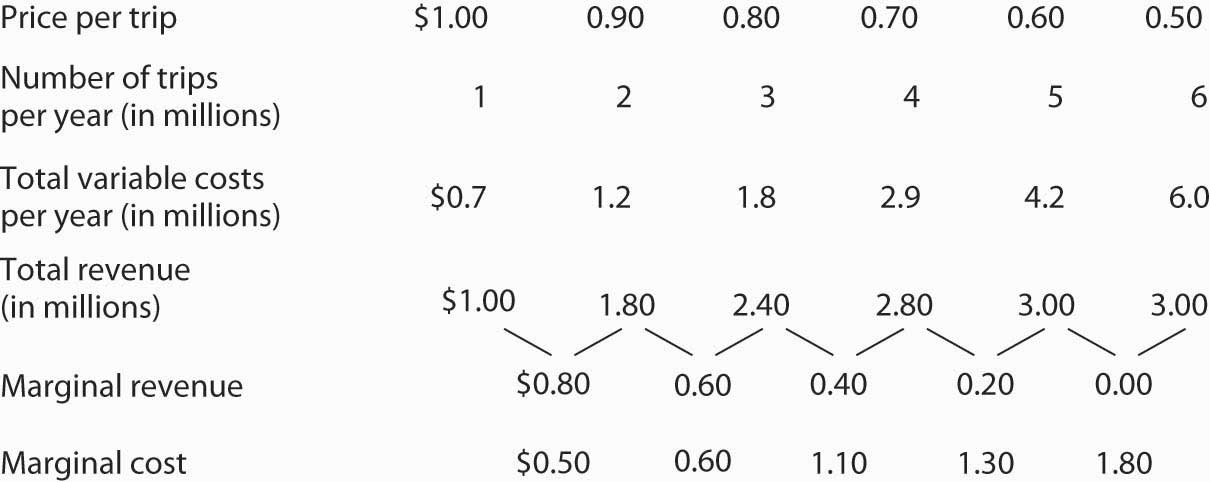
Maintenance costs institute the variable costs associated with building the road. In order to answer the first iv parts of the question, you volition demand to compute total revenue, marginal acquirement, and marginal cost, as shown at right:

1. Using the "midpoint" convention, the profit-maximizing level of output is 2.5 million trips per year. With that number of trips, marginal revenue ($0.60) equals marginal cost ($0.60).
2. Over again, we apply the "midpoint" convention. The company volition charge a toll of $0.85.
3. The marginal revenue is $0.60, which is less than the $0.85 cost (toll).

blevinssidied1947.blogspot.com

Source: https://saylordotorg.github.io/text_principles-of-economics-v2.0/s13-02-the-monopoly-model.html

Share this post